Summary

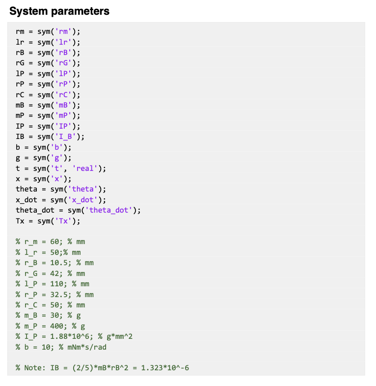
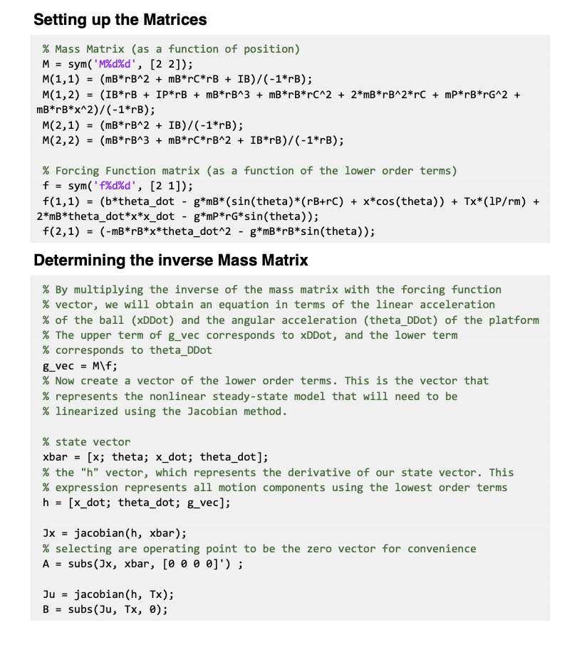
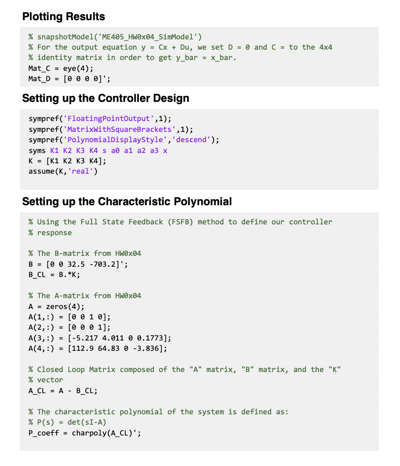
In preparation of our term project and to continue to build off of HW 0x02 and HW 0x04, we developed a closed loop controller for our system model. To ensure consistency and accuracy of our system, we decided to pursue the MatLab/Simulink tools in order to complete our assignment. You will find our Matlab and Simulink documentation below.

Engineering Requirements

• Determine 1x4 gain vector K = [K1, K2, K3, K4]
• Define a method of determining pole locations based criteria
• Find the characteristic polynomial associated with selected pole locations
• Determine the gains K1 through K4.

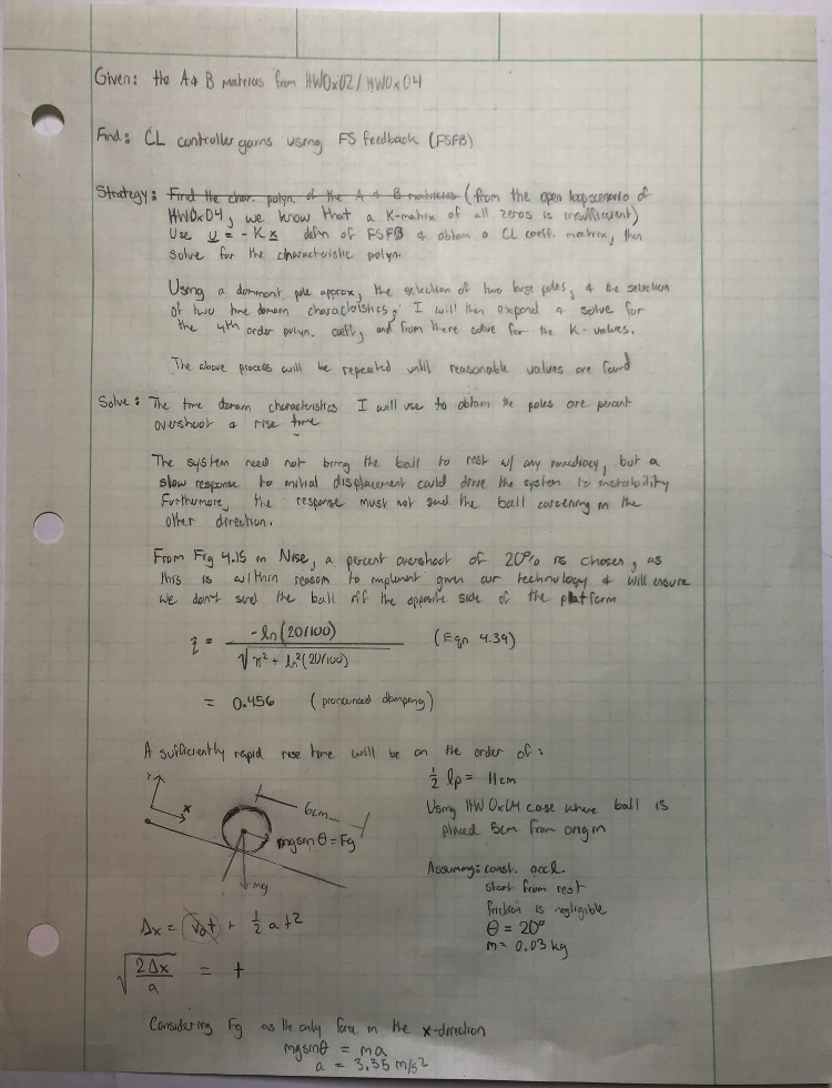
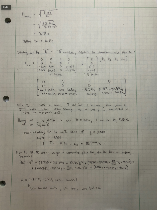
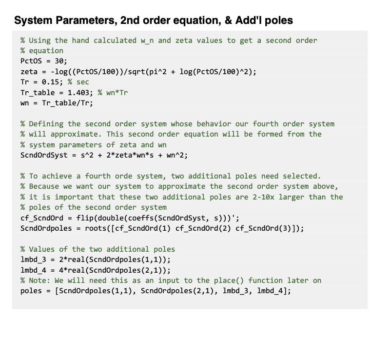
Method of determining pole locations based on criteria was making a dominant pole approximation and choosing two large poles along with two time-domain characteristics like settling time and overshoot percentage.

Hand Calculations

Matlab and Simulink

HW 0x05: Developing a Closed Loop Control System for the Balancing Platform

Figure 1. Simulink Model

Results

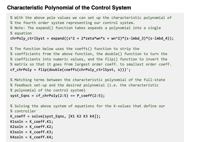
Verify K values using place() command

Figure 2. Compared calculated results versus results found via place() command

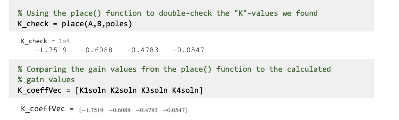
As you can see in Figure 1, the values we outputted matched that of the values resulting from the use of the place() command.

Figure 3. HW 0x04 Controller Plots

Figure 3. HW 0x05 Controller Plots

Discussion & Analysis

1. Show confirmation that your calculated gains correctly place the closed-loop poles at your desired locations

Setting and iterating upon the parameters of rise time and percent overshoot, we arrive at gain values after solving the system characteristic polynomial for the values of "K". When using the place() function to compare the calculated gains to that calculated using the place() function (see attached MATLAB code), we see identical results between the two, with the values being: [-1.7159 -0.6088 -0.4783 -0.547].

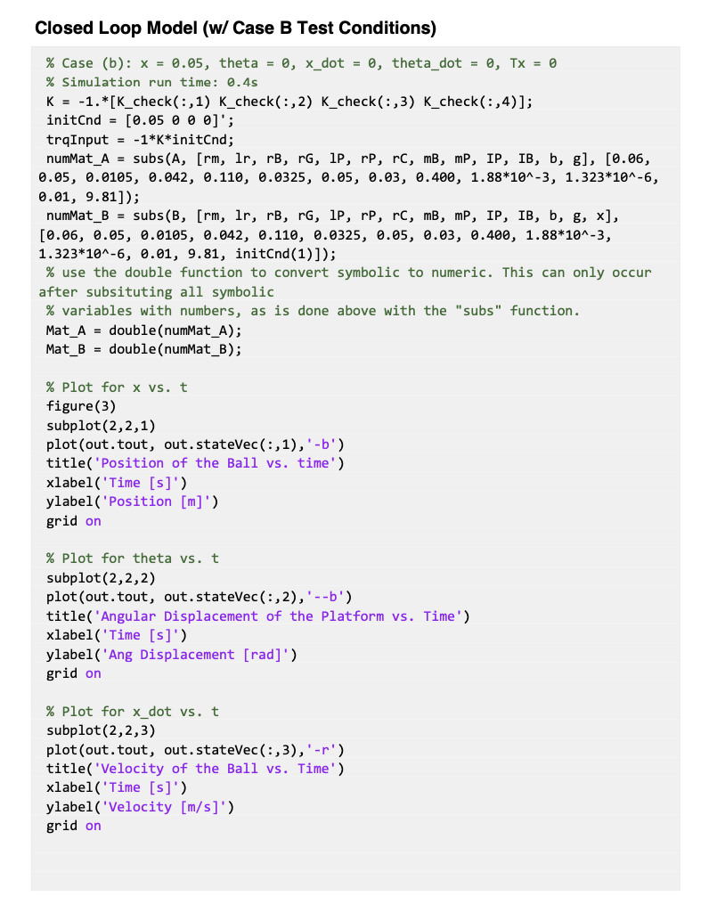
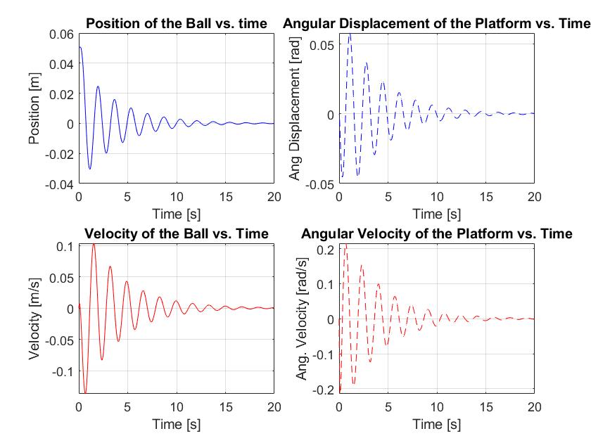
2. Show your tuned closed-loop simulation results and comment on the differences (hopefully positive ones) compared to the closed-loop response in HW 0x04.

From inspection, the tuned open-loop system has a smaller settling time, rise time and percent overshoot. Accomplishing such variations involved increasing the value of the damping ratio (zeta) which increased the value of the real term, driving percent overshoot and settling time down. Additionally, but to a lesser extent, the increase of the damping ratio and increase of the natural frequency drove the rise time up as well. These differences illustrate a more effective controller, one that reaches equilibrium sooner, that responds to the ball's placement quicker, and exhibits more controlled motion.

3. Comment on the performance of your system: Did you achieve the criteria that you selected?

In order to compare percent overshoot values between the HW0x04 controller and the HW0x05 controller design above, I used the min function to obtain minimum (negative) values as these correspond to the actual peak. The HW0x04 controller exhibited a peak of -0.03048 [m], whereas the HW0x05 controller exhibited a peak of -0.0068 [m]. Given the large difference between the values and that they both share the same steady state value, the explicit OS comparison is unnecessary. Additionally, using the damping ratio and natural frequency values of the HW0x05 controller, we get a settling time of 1.195 [s], which can be observed as being far less than that of the HW0x04 controller. Finally, using peak time as opposed to rise time calculations because they both would exhibit similar trend (and for the sake of parsimony), we find the peak time of the HW0x05 controller to be 0.5638 [s], as compared to the 1.142 [s] value of the HW0x04 controller.